Example 2 - Compute Curie depth
Bouligand et al. (2009) model the crust as a layer between depths \(z_t\) and \(z_t + \Delta z\) whose magnetisation is fractal rather than spatially random, with a fractal parameter \(\beta\). The radially averaged power spectrum of the anomaly is then
where \(A\) collects a \(\cosh\) and a modified Bessel function of \(|k|\Delta z\), and \(C\) is a constant setting the overall level. pycurious.bouligand2009 evaluates the whole expression.
Unlike the centroid method of Tanaka, which takes two limits of a simpler layer model and fits a straight line to each, this is fitted whole, over the entire spectrum at once, for all four parameters together. Two consequences follow, and they are the reason to prefer it:
there are no bands to choose, and so no chance of fitting outside the range where an approximation holds;
\(\beta\) is estimated from the data rather than assumed, so a fractal source introduces no bias to be corrected for afterwards.
The Curie point depth is then simply the base of the layer,
This notebook generates an anomaly whose parameters we choose, so that every number below can be checked against a known answer.
Contents
import numpy as np
import matplotlib.pyplot as plt
%matplotlib inline

import pycurious
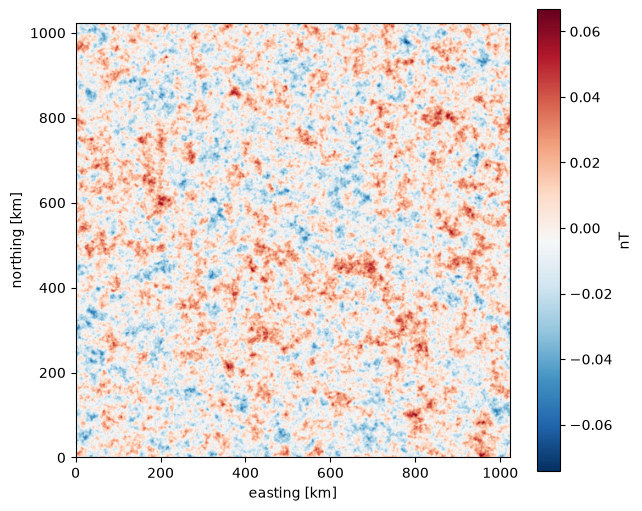
A synthetic with a known answer
pycurious.fractal_anomaly filters white noise by the square root of equation (1), so the expected power spectrum of the result is the model, for whichever \(\beta\), \(z_t\) and \(\Delta z\) we ask for.
Here the source runs from 1 km down to 21 km, so the Curie depth we are trying to recover is 21 km.
beta_true, zt_true, dz_true = 3.0, 1.0, 20.0

data, extent = pycurious.fractal_anomaly(
    n=512, dx=2.0, beta=beta_true, zt=zt_true, dz=dz_true, C=5.0, seed=1)

grid = pycurious.CurieOptimiseBouligand(data, *extent)

xpt = 0.5*(extent[0] + extent[1])
ypt = 0.5*(extent[2] + extent[3])
window_size = 1000e3

print("grid is {:.0f} km across at {:.0f} km spacing".format(
    (extent[1] - extent[0])*1e-3, grid.dx*1e-3))
print("true Curie depth = {:.1f} km".format(zt_true + dz_true))
grid is 1022 km across at 2 km spacing
true Curie depth = 21.0 km
fig, ax = plt.subplots(figsize=(7, 6))
im = ax.imshow(data, extent=np.array(extent)*1e-3, cmap='RdBu_r', origin='lower')
ax.set_xlabel('easting [km]')
ax.set_ylabel('northing [km]')
fig.colorbar(im, ax=ax, label='nT')
plt.show()
The radial power spectrum
window_spectrum extracts a square window, computes the radially averaged spectrum, and returns the uncertainty of each binned value ready for fitting. That last part is not the scatter of the FFT cells within an annulus, which is what radial_spectrum reports: it is the uncertainty of their mean, deflated because the cells are not independent of one another.
power=2 gives \(\ln \Phi_{\Delta T}\), the log power spectrum that equation (1) describes. Wavenumbers come back in rad/km.
k, Phi, sigma_Phi = grid.window_spectrum(
    window_size, xpt, ypt, taper=np.hanning, power=2.0)

print("{} bins, from {:.4f} to {:.3f} rad/km".format(len(k), k.min(), k.max()))
print("wavelengths {:.1f} km down to {:.1f} km".format(2*np.pi/k.min(), 2*np.pi/k.max()))
249 bins, from 0.0076 to 1.564 rad/km
wavelengths 830.1 km down to 4.0 km
Fitting the four parameters
optimise returns each parameter followed by its standard deviation. The uncertainties come from the curvature of the misfit at the solution, corrected for the fact that neighbouring spectral bins are correlated — a taper spreads each wavenumber over a main lobe several bins wide, and ignoring that would make every error bar about 30% too narrow.
beta, zt, dz, C, sigma_beta, sigma_zt, sigma_dz, sigma_C = grid.optimise(
    window_size, xpt, ypt, taper=np.hanning)

print("             recovered            true")
print("beta    {:8.3f} +/- {:5.3f}   {:8.3f}".format(beta, sigma_beta, beta_true))
print("z_t     {:8.3f} +/- {:5.3f}   {:8.3f}".format(zt, sigma_zt, zt_true))
print("dz      {:8.3f} +/- {:5.3f}   {:8.3f}".format(dz, sigma_dz, dz_true))
print("C       {:8.3f} +/- {:5.3f}        --".format(C, sigma_C))
             recovered            true
beta       3.020 +/- 0.056      3.000
z_t        0.986 +/- 0.035      1.000
dz        23.324 +/- 3.763     20.000
C          2.398 +/- 0.069        --
\(\beta\) and \(z_t\) come back within a standard deviation of the truth. \(\Delta z\) is high by 3.5 km, rather more than its own error bar suggests, and that is the honest behaviour of this parameter rather than a failure — we return to it below.
\(C\) has no true value to compare against. It is a level rather than a depth, and absorbs every constant between the noise and the spectrum: the generator normalises out the grid size, but the log-averaging of the spectrum and the power a taper removes both remain, leaving it about 2.5 low. Treat it as a nuisance parameter.
fig, ax = plt.subplots(figsize=(9, 6))

ax.errorbar(k, Phi, yerr=sigma_Phi, fmt='o', ms=3, color='C0',
            elinewidth=0.8, label='measured spectrum')
ax.plot(k, pycurious.bouligand2009(k, beta, zt, dz, C), 'r-', lw=2,
        label='fit')
ax.plot(k, pycurious.bouligand2009(k, beta_true, zt_true, dz_true, C), 'k--', lw=1.5,
        label='true parameters')

ax.set_xlabel(r'$|k|$ [rad km$^{-1}$]')
ax.set_ylabel(r'$\ln \Phi_{\Delta T}$')
ax.legend()
plt.show()
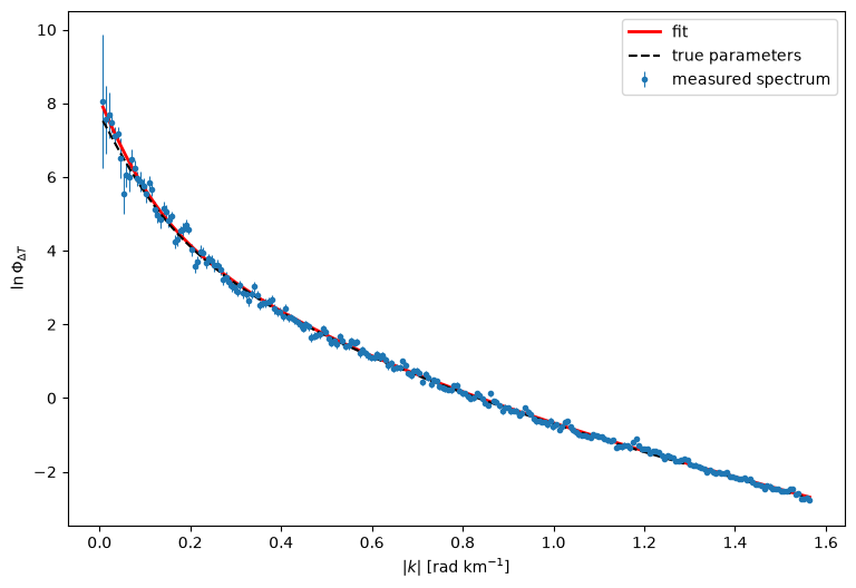
The fit and the truth are hard to tell apart, which is the point: over most of the spectrum a 17% error in \(\Delta z\) is nearly invisible. Only the handful of longest-wavelength bins on the left carry information about the base of the layer, because that is where the \(|k|\Delta z\) terms in equation (1) are of order one.
That is the whole difficulty of the method, and it is worth seeing plotted rather than described.
An honest interval on the Curie depth
calculate_CPD applies equation (2) and combines the two uncertainties in quadrature.
CPD, sigma_CPD = grid.calculate_CPD(zt, dz, sigma_zt, sigma_dz)

print("Curie depth = {:.2f} +/- {:.2f} km   (true {:.1f} km)".format(
    CPD, sigma_CPD, zt_true + dz_true))
Curie depth = 24.31 +/- 3.76 km (true 21.0 km)
That \(\pm\) is symmetric, and the Curie depth is not. The likelihood in \(\Delta z\) has a long upper tail (Mather & Fullea, 2019): a layer thicker than the data can resolve looks much like one that is merely thick, whereas a much thinner one does not fit at all. So the plausible values run further above the estimate than below it, and a symmetric error bar describes neither end well.
profile scans one quantity, re-optimising everything else at each step, and reports where the misfit rises by the \(\chi^2\) threshold for the requested confidence. It makes no assumption of symmetry. Asking it for "CPD" profiles the Curie depth directly, by substituting \(\Delta z = Z_b - z_t\), rather than propagating a symmetric \(\sigma_{\Delta z}\) through equation (2).
values, deviance, lower, upper = grid.profile(
    window_size, xpt, ypt, "CPD", level=0.95, taper=np.hanning)

print("profile 95%    [{:6.2f}, {:6.2f}] km".format(lower, upper))
print("symmetric 95%  [{:6.2f}, {:6.2f}] km".format(
    CPD - 1.96*sigma_CPD, CPD + 1.96*sigma_CPD))
print("true value     {:6.2f} km".format(zt_true + dz_true))
profile 95%    [ 19.66,  31.22] km
symmetric 95%  [ 16.93,  31.68] km
true value      21.00 km
fig, ax = plt.subplots(figsize=(9, 5))

ax.plot(values, deviance, 'C0-', lw=2)
ax.axhline(3.84, color='k', ls='--', lw=1, label=r'95% threshold, $\chi^2_1$')
ax.axvspan(lower, upper, color='C0', alpha=0.15, label='95% interval')
ax.axvline(zt_true + dz_true, color='r', lw=2, label='true Curie depth')

ax.set_xlabel('Curie depth [km]')
ax.set_ylabel(r'deviance  $2(F - F_{min})$')
ax.set_ylim(0, 15)
ax.legend()
plt.show()
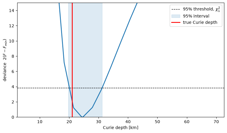
The curve is visibly steeper on the left than on the right, and the interval inherits that: it reaches 7.0 km above the estimate but only 4.7 km below. The true value sits comfortably inside.
Note what the symmetric interval got wrong. Its upper end is close to the profile’s, but its lower end reaches down to 17 km — a Curie depth the data actually rule out. Reporting \(\pm\sigma\) here would understate how well the shallow side is constrained while understating how far the deep side can reach.
How wide a window?
Only the longest wavelengths constrain \(\Delta z\), and a window can only resolve wavelengths up to its own size. So the window has to be several times the depth being sought, and the consequence of ignoring that is severe.
windows = np.array([300e3, 500e3, 700e3, 1000e3])

print(" window      dz +/- sigma        CPD")
results = []
for w in windows:
    o = grid.optimise(w, xpt, ypt, taper=np.hanning)
    results.append(o)
    print("{:5.0f} km   {:6.2f} +/- {:6.2f}   {:6.2f}".format(
        w*1e-3, o[2], o[6], o[1] + o[2]))
 window      dz +/- sigma        CPD
  300 km    46.73 +/-  69.72    47.72
  500 km    30.35 +/-  10.97    31.34
  700 km    25.54 +/-   6.52    26.51
 1000 km    23.32 +/-   3.76    24.31
fig, (ax1, ax2) = plt.subplots(1, 2, figsize=(13, 5))

dz_fit = np.array([o[2] for o in results])
dz_err = np.array([o[6] for o in results])
beta_fit = np.array([o[0] for o in results])
beta_err = np.array([o[4] for o in results])

ax1.errorbar(windows*1e-3, dz_fit, yerr=dz_err, fmt='o-', capsize=4)
ax1.axhline(dz_true, color='k', ls='--', label=r'true $\Delta z$')
ax1.set_ylabel(r'$\Delta z$ [km]')
ax1.legend()

ax2.errorbar(windows*1e-3, beta_fit, yerr=beta_err, fmt='o-', capsize=4, color='C1')
ax2.axhline(beta_true, color='k', ls='--', label=r'true $\beta$')
ax2.set_ylabel(r'$\beta$')
ax2.legend()

for ax in (ax1, ax2):
    ax.set_xlabel('window size [km]')
plt.show()
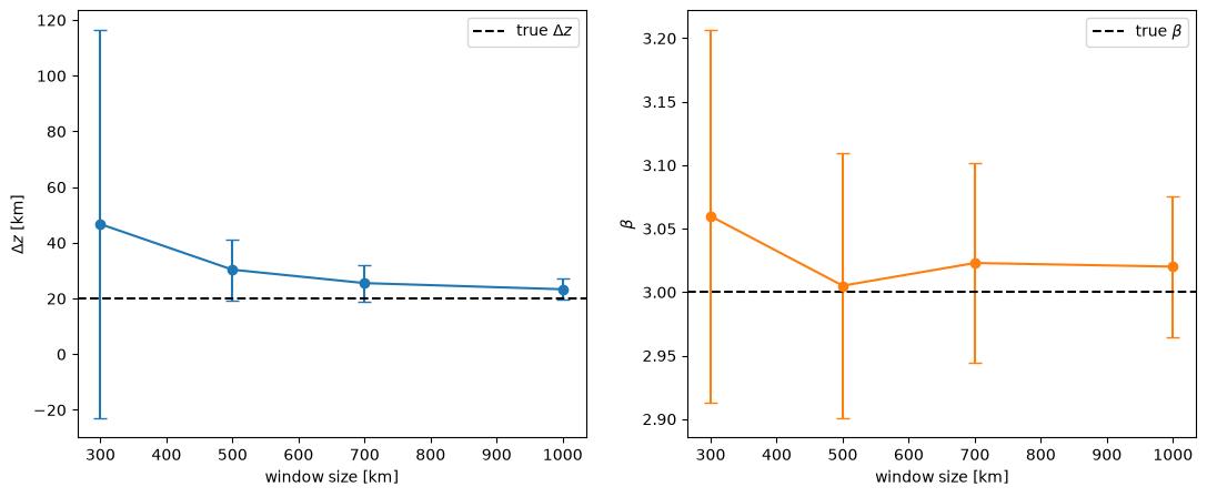
\(\beta\) is recovered at every window size, because it is set by the slope of the spectrum across the whole wavenumber range and a small window still resolves that. \(\Delta z\) is not: at 300 km it comes back at 46 km against a true 20, more than twice the answer.
But look at the error bar it reports — \(\pm 67\) km. The fit is not quietly wrong; it says plainly that it cannot constrain the parameter. That is the practical value of carrying uncertainties through: a 300 km window over a 21 km Curie depth produces a number that must not be believed, and the number itself tells you so.
Suggestion: use a window at least 10 times the expected Curie depth, and read the reported \(\sigma_{\Delta z}\) before trusting the result.
Adding a prior
Where the data cannot constrain a parameter, independent knowledge can. add_prior accepts a mean and standard deviation, or any frozen distribution from scipy.stats, and the prior enters the fit as one additional observation.
\(\beta\) for continental crust is often taken to be near 3, so it is the natural candidate.
grid.add_prior(beta=(3.0, 0.05))
constrained = grid.optimise(window_size, xpt, ypt, taper=np.hanning)
grid.reset_priors()

print("                 no prior      beta prior")
print("beta      {:12.3f}    {:12.3f}".format(beta, constrained[0]))
print("dz        {:12.3f}    {:12.3f}".format(dz, constrained[2]))
print("sigma_dz  {:12.3f}    {:12.3f}".format(sigma_dz, constrained[6]))
                 no prior      beta prior
beta             3.020           3.012
dz              23.324          23.699
sigma_dz         3.763           3.295
Pinning \(\beta\) tightens \(\sigma_{\Delta z}\) from 3.7 to 3.3 km. The improvement is real but modest, which is itself informative: \(\beta\) and \(\Delta z\) are not so strongly traded off against each other that fixing one determines the other. A prior on \(\beta\) is not a substitute for a window wide enough to see the base of the layer.
Summary
Fit the whole spectrum at once. There are no bands to choose, and \(\beta\) is estimated rather than assumed.
Use a window at least ten times the expected Curie depth. \(\beta\) and \(z_t\) survive a small window; \(\Delta z\) does not.
Read \(\sigma_{\Delta z}\). When the window is too small it becomes large enough to disqualify the estimate, which is the fit telling you the truth.
Report the Curie depth with
profile, not \(\pm\sigma\). Its uncertainty is genuinely asymmetric, and the symmetric interval misdescribes both ends.
References
Bouligand, C., Glen, J. M. G., & Blakely, R. J. (2009). Mapping Curie temperature depth in the western United States with a fractal model for crustal magnetization. Journal of Geophysical Research, 114, B11104. doi:10.1029/2009JB006494
Mather, B., & Fullea, J. (2019). Constraining the geotherm beneath the British Isles from Bayesian inversion of Curie depth: integrated modelling of magnetic, geothermal, and seismic data. Solid Earth, 10, 839-850. doi:10.5194/se-10-839-2019