Example 3 - Parameter Exploration

The Curie depth returned by the centroid method depends on three choices the user makes: where in \(k\)-space each fitting band sits, how wide those bands are, and how large a window of magnetic data is used. None of these is determined by the data, so it is worth knowing how much they matter.

CurieOptimiseTanaka.optimise reports an uncertainty from the fit covariance, which captures the scatter of the spectrum but not the sensitivity to these choices. The sweeps below explore that sensitivity directly.

Bands are specified in rad/km. Where the original version of this notebook used spatial frequency in cycles/km, the values are multiplied by \(2\pi\).

Contents

1. Where in \(k\)-space the bands sit

2. How wide the bands are

3. How large the data window is

import numpy as np
import matplotlib.pyplot as plt
%matplotlib inline

import pycurious

# load x,y,anomaly
mag_data = np.loadtxt("../../data/test_mag_data.txt")

nx, ny = 305, 305

x = mag_data[:,0]
y = mag_data[:,1]
d = mag_data[:,2].reshape(ny,nx)

xmin, xmax = x.min(), x.max()
ymin, ymax = y.min(), y.max()

# initialise object
grid = pycurious.CurieOptimiseTanaka(d, xmin, xmax, ymin, ymax)

# pick centroid
xpt = xmin + (xmax-xmin)/2
ypt = ymin + (ymax-ymin)/2

Varying spatial frequency range

This test explores where in \(k\)-space is specific window used, separately for both the power and \(k\)-weighted power.

# 1) Where in k-space do we locate the bands?
import warnings

window_size = 304e3
band_width = 2*np.pi*0.1

zt_array = 2*np.pi*np.arange(0.0, 0.5, 0.05)
z0_array = 2*np.pi*np.arange(0.0, 0.5, 0.05)

z0q, ztq = np.meshgrid(z0_array, zt_array)

CPD_grid       = np.full((zt_array.size, z0_array.size), np.nan)
sigma_CPD_grid = np.full((zt_array.size, z0_array.size), np.nan)

# the sweep deliberately visits bands that are too low or too sparse to fit,
# so suppress the band warnings and record those as NaN
with warnings.catch_warnings():
    warnings.simplefilter("ignore")

    for row, zt_min in enumerate(zt_array):
        for col, z0_min in enumerate(z0_array):
            try:
                zt, z0, zt_int, z0_int, sigma_zt, sigma_z0 = grid.optimise(
                    window_size, xpt, ypt,
                    (zt_min, zt_min + band_width),
                    (z0_min, z0_min + band_width),
                    taper=None)
            except ValueError:
                continue

            CPD, sigma_CPD = grid.calculate_CPD(zt, z0, sigma_zt, sigma_z0)
            CPD_grid[row, col] = CPD
            sigma_CPD_grid[row, col] = sigma_CPD

print("{} of {} band combinations produced a fit".format(
    np.isfinite(CPD_grid).sum(), CPD_grid.size))

100 of 100 band combinations produced a fit

fig, (ax1, ax2) = plt.subplots(1, 2, figsize=(14,5.5))

sc1 = ax1.scatter(ztq.flat, z0q.flat, c=CPD_grid.flat, s=260, marker='s')
fig.colorbar(sc1, ax=ax1, label='CPD [km]')
ax1.set_xlabel(r'$Z_t$ band start [rad km$^{-1}$]')
ax1.set_ylabel(r'$Z_o$ band start [rad km$^{-1}$]')
ax1.set_title('Curie depth')

sc2 = ax2.scatter(ztq.flat, z0q.flat, c=sigma_CPD_grid.flat, s=260, marker='s')
fig.colorbar(sc2, ax=ax2, label='CPD stdev [km]')
ax2.set_xlabel(r'$Z_t$ band start [rad km$^{-1}$]')
ax2.set_ylabel(r'$Z_o$ band start [rad km$^{-1}$]')
ax2.set_title('Reported uncertainty')

plt.show()

print("CPD ranges from {:.1f} to {:.1f} km across these bands (true value 10.3 km),".format(
    np.nanmin(CPD_grid), np.nanmax(CPD_grid)))
print("while the reported uncertainty is at most {:.1f} km.".format(np.nanmax(sigma_CPD_grid)))

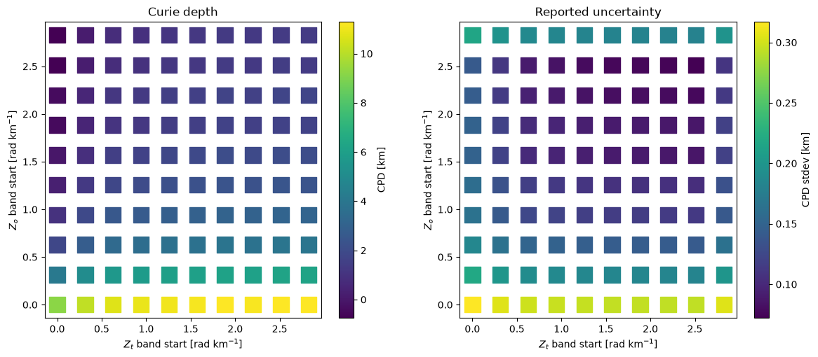
CPD ranges from -0.8 to 11.3 km across these bands (true value 10.3 km),
while the reported uncertainty is at most 0.3 km.

The spread across band positions is far larger than any individual error bar. That is the central caveat of the method: the uncertainty returned by optimise describes the scatter of the spectrum about a line, not whether the line was fitted in the right place.

Varying the bandwidth

Widening a band brings in more spectral estimates and stabilises the gradient, at the cost of fitting a straight line across a curve that is not straight.

# 2) How wide a band in k-space do we want?

nbins = 30
bandwidths = 2*np.pi*np.linspace(0.05, 0.1, nbins)

CPD_grid       = np.full(nbins, np.nan)
sigma_CPD_grid = np.full(nbins, np.nan)

zt_min = 2*np.pi*0.2
z0_min = 0.0

with warnings.catch_warnings():
    warnings.simplefilter("ignore")

    for i, bandwidth in enumerate(bandwidths):
        try:
            zt, z0, zt_int, z0_int, sigma_zt, sigma_z0 = grid.optimise(
                window_size, xpt, ypt,
                (zt_min, zt_min + bandwidth),
                (z0_min, z0_min + bandwidth),
                taper=None)
        except ValueError:
            continue

        CPD_grid[i], sigma_CPD_grid[i] = grid.calculate_CPD(
            zt, z0, sigma_zt, sigma_z0)

fig, ax2 = plt.subplots(figsize=(8,6))
ax2.errorbar(bandwidths, CPD_grid, yerr=sigma_CPD_grid, capsize=3)
ax2.axhline(10.305, color='k', linestyle='--', label='true Curie depth')
ax2.invert_yaxis()
ax2.set_xlabel(r'Bandwidth $k_{max} - k_{min}$ [rad km$^{-1}$]')
ax2.set_ylabel('CPD [km]')
ax2.legend()
plt.show()

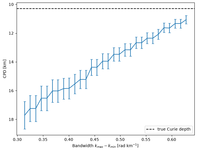
The estimate settles down once the band is wide enough to contain a reasonable number of spectral estimates. Widening it further keeps shrinking the error bar, but that shrinkage is misleading: the spectrum is not truly linear over a wide range of \(k\), so a wider band trades random error for systematic error.

Varying window size

The window controls the spectral resolution, \(\Delta k = 2\pi / (N \Delta x)\). A narrow window gives few long-wavelength bins, which is exactly what the centroid fit depends on.

# 3) How large a window of magnetic data is required?

n_windows = 50
window_sizes = np.linspace(50e3, 304e3, n_windows)

zt_range = (2*np.pi*0.2, 2*np.pi*0.3)
z0_range = (0.0, 2*np.pi*0.1)

CPD_grid       = np.full(n_windows, np.nan)
sigma_CPD_grid = np.full(n_windows, np.nan)

with warnings.catch_warnings():
    warnings.simplefilter("ignore")

    for i, window in enumerate(window_sizes):
        try:
            zt, z0, zt_int, z0_int, sigma_zt, sigma_z0 = grid.optimise(
                window, xpt, ypt, zt_range, z0_range, taper=None)
        except ValueError:
            continue

        CPD_grid[i], sigma_CPD_grid[i] = grid.calculate_CPD(
            zt, z0, sigma_zt, sigma_z0)

fig, ax1 = plt.subplots(figsize=(8,6))
ax1.errorbar(window_sizes/1e3, CPD_grid, yerr=sigma_CPD_grid, capsize=3)
ax1.axhline(10.305, color='k', linestyle='--', label='true Curie depth')
ax1.set_xlabel('Window size [km]')
ax1.set_ylabel('CPD [km]')
ax1.legend()
plt.show()

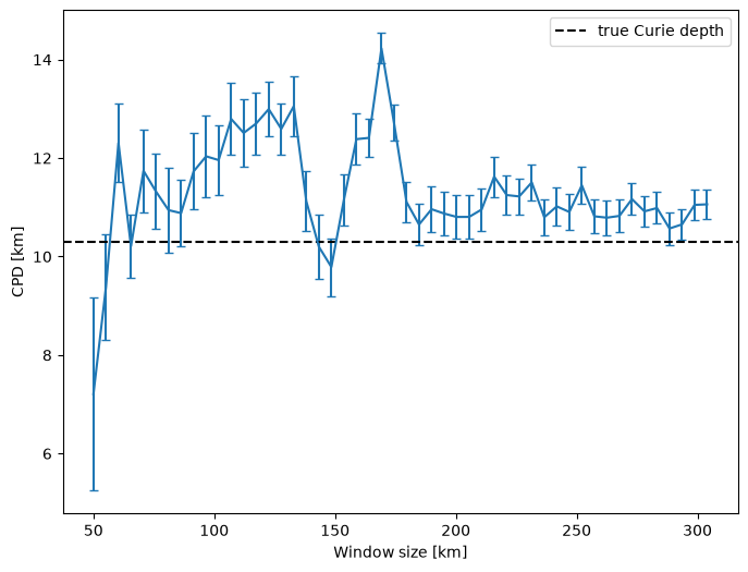
There is considerable scatter at every window size, so a range of windows should be tested for any dataset rather than trusting a single one. The reported uncertainty does shrink as the window grows, since a finer \(\Delta k\) puts more spectral estimates into each band.

Be careful how much comfort to take from that. A larger window narrows the error bar whether or not the bands are valid, and on this 305 km grid the \(Z_o\) band never satisfies \(|k|d \ll 1\) — see Ex2. Precision and accuracy are not the same thing here.