Example 1 - Plot amplitude spectra

PyCurious offers convenience functions to extract the radial amplitude spectrum. This has been covered in the Bouligand folder of jupyter notebooks and is largely duplicated here.

In this notebook we plot the amplitude power spectrum using the analytical expression, and the spectrum computed from a synthetic magnetic anomaly. (This can be generated from Bouligand_forward.py in the tests directory.)

Contents

• Radial amplitude spectrum

import numpy as np
import matplotlib.pyplot as plt
%matplotlib inline

import pycurious

Radial amplitude spectrum

The radial amplitude spectrum is computed from a square window of the magnetic anomaly. Methods to select window sizes and compute the Fast Fourier Transform (FFT) belong to the CurieGrid object.

CurieGrid achieves the following purposes:

• Upward continuation

• Reduction to the pole

• Compute the radial amplitude spectrum using FFT

The shape of the radial amplitude spectrum is heavily dependent on window size. Resolution of long wavelength features require large windows.

Suggestion: use a window size > 4 times the maximum Curie depth.

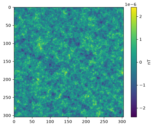
# load magnetic anomaly - i.e. random fractal noise
mag_data = np.loadtxt("../../data/test_mag_data.txt")

nx, ny = 305, 305

x = mag_data[:,0]
y = mag_data[:,1]
d = mag_data[:,2].reshape(ny,nx)

xmin, xmax = x.min(), x.max()
ymin, ymax = y.min(), y.max()

## Plot random fractal noise

fig = plt.figure()
ax1 = fig.add_subplot(111)
im1 = ax1.imshow(d)
fig.colorbar(im1, label='nT')

<matplotlib.colorbar.Colorbar at 0x7feadce4f8c0>

# initialise CurieGrid object
grid = pycurious.CurieGrid(d, xmin, xmax, ymin, ymax)

# pick the centroid
xpt = 0.5*(xmin + xmax)
ypt = 0.5*(ymin + ymax)

window_size = 304e3
subgrid = grid.subgrid(window_size, xpt, ypt)

Amplitude or power?

radial_spectrum raises the FFT of the anomaly to power before averaging, so the two Curie depth methods in PyCurious ask for different values:

method	power	quantity returned
Bouligand et al. (2009)	2 (default)	\(\ln \Phi_{\Delta T}\), the log power spectrum
Tanaka et al. (1999)	1	\(\ln \Phi_{\Delta T}^{1/2}\), the log amplitude spectrum

Tanaka’s equations are written in terms of the amplitude spectrum \(\Phi_{\Delta T}^{1/2}\), and because \(\Phi_{\Delta T} = |\mathrm{FFT}|^2\), that is power=1. Getting this wrong rescales every depth the method returns.

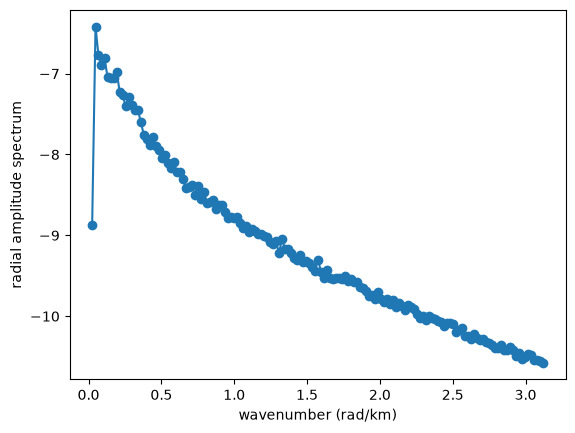
# compute radial power spectrum
k, Phi, sigma_Phi = grid.radial_spectrum(subgrid, taper=None, power=1)

# plot radial power spectrum
fig = plt.figure()
ax1 = fig.add_subplot(111, xlabel="wavenumber (rad/km)", ylabel="radial amplitude spectrum")
ax1.plot(k, Phi, '-o')
plt.show()

Choice of taper

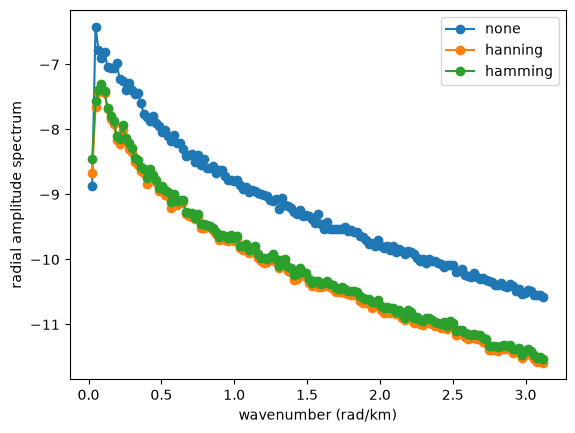
The default taper is the hanning filter (see numpy.hanning for more details), but other functions can be passed to taper, or simply set it to None. There is a significant offset in the amplitude spectrum with tapering functions, however, it is the slope of the spectrum with wavenumber that is most important when it comes to determining Curie depth.

k1, Phi1, sigma_Phi1 = grid.radial_spectrum(subgrid, taper=None, power=1)
k2, Phi2, sigma_Phi2 = grid.radial_spectrum(subgrid, taper=np.hanning, power=1)
k3, Phi3, sigma_Phi2 = grid.radial_spectrum(subgrid, taper=np.hamming, power=1)


fig = plt.figure()
ax1 = fig.add_subplot(111, xlabel="wavenumber (rad/km)", ylabel="radial amplitude spectrum")
ax1.plot(k1, Phi1, '-o', label='none')
ax1.plot(k2, Phi2, '-o', label='hanning')
ax1.plot(k3, Phi3, '-o', label='hamming')
ax1.legend()
plt.show()