Example 3 - Posing the inverse problem

Ex2 fitted four parameters and reported a standard deviation for each. This notebook asks where those uncertainties come from, and how far to trust them.

Fitting the spectrum is a Bayesian inverse problem. Writing \(\mathbf{m} = (\beta, z_t, \Delta z, C)\) for the parameters and \(\Phi_d\) for the observed spectrum,

\[(1) \quad P(\mathbf{m}|\Phi_d) \propto P(\Phi_d|\mathbf{m}) \, P(\mathbf{m})\]

With Gaussian errors on each spectral bin the negative log of the right-hand side is

\[(2) \quad F(\mathbf{m}) = \frac{1}{2}\sum_i \left( \frac{\Phi(|k_i|, \mathbf{m}) - \Phi_{d,i}}{\sigma_i} \right)^2 \; + \; \frac{1}{2}\sum_j \left( \frac{m_j - p_j}{\sigma_{p_j}} \right)^2\]

which is what min_func returns. The first sum is the data misfit; the second adds one term per prior, so a Gaussian prior is simply one more observation. Minimising \(F\) gives the most probable model, and the shape of \(F\) around that minimum gives the uncertainty.

There are four ways to characterise that shape, and they cost very different amounts. This notebook runs all four on the same data, and ends with the reason they must not be used to check one another.

Contents

• The misfit surface

• 1. The fit covariance

• 2. Profile likelihood

• 3. Resampling the spectrum

• 4. Markov chain Monte Carlo

• Why agreement is not validation

import numpy as np
import matplotlib.pyplot as plt
from scipy import stats
%matplotlib inline

import pycurious

beta_true, zt_true, dz_true = 3.0, 1.0, 20.0
CPD_true = zt_true + dz_true

data, extent = pycurious.fractal_anomaly(
    n=512, dx=2.0, beta=beta_true, zt=zt_true, dz=dz_true, C=5.0, seed=1)

grid = pycurious.CurieOptimiseBouligand(data, *extent)

xpt = 0.5*(extent[0] + extent[1])
ypt = 0.5*(extent[2] + extent[3])
window_size = 1000e3

k, Phi, sigma_Phi = grid.window_spectrum(
    window_size, xpt, ypt, taper=np.hanning, power=2.0)

The misfit surface

Equation (2) over the two parameters that are hardest to separate, with \(z_t\) and \(C\) held at their fitted values.

*fit, cov = grid.optimise(window_size, xpt, ypt, taper=np.hanning,
                          return_cov=True)
beta, zt, dz, C = fit[:4]
sigma_beta, sigma_zt, sigma_dz, sigma_C = fit[4:]

nb = 60
beta_range = np.linspace(beta - 0.25, beta + 0.25, nb)
dz_range = np.linspace(max(dz - 15.0, 1.0), dz + 25.0, nb)

misfit = np.array([[grid.min_func([b, zt, d, C], k, Phi, sigma_Phi)
                    for d in dz_range] for b in beta_range])

fig, (ax1, ax2) = plt.subplots(1, 2, sharey=True, figsize=(13, 5))
X, Y = np.meshgrid(dz_range, beta_range)

im1 = ax1.pcolormesh(X, Y, misfit, shading='auto')
im2 = ax2.pcolormesh(X, Y, np.exp(-(misfit - misfit.min())), shading='auto')

for ax in (ax1, ax2):
    ax.scatter(dz, beta, c='r', s=40, zorder=5, label='best fit')
    ax.scatter(dz_true, beta_true, c='w', s=40, marker='x', zorder=5, label='truth')
    ax.set_xlabel(r'$\Delta z$ [km]')
    ax.legend()

ax1.set_ylabel(r'$\beta$')
ax1.set_title(r'misfit $F(\mathbf{m})$')
ax2.set_title(r'$P(\mathbf{m}|\Phi_d) \propto e^{-F}$')
fig.colorbar(im1, ax=ax1)
fig.colorbar(im2, ax=ax2)
plt.show()

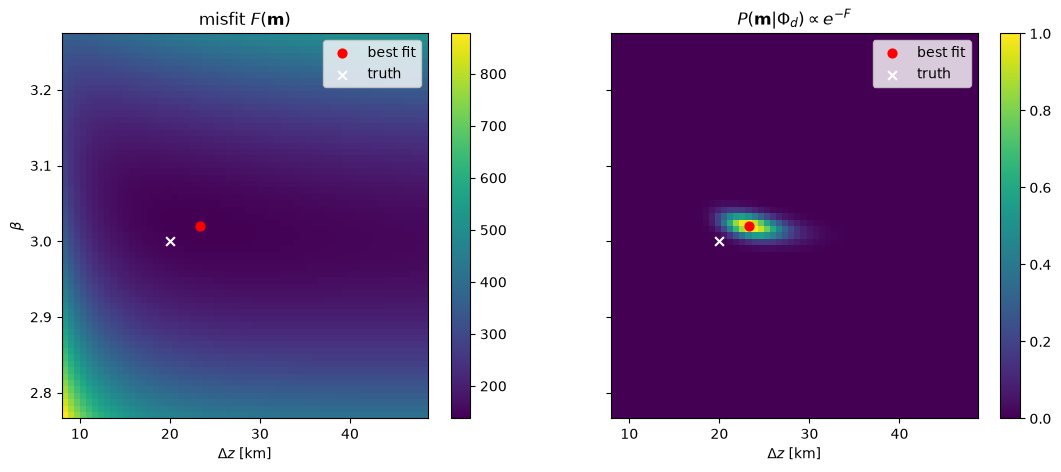
The probability is a narrow ridge, not a round hill. It is tight in \(\beta\), slack in \(\Delta z\), tilted because the two trade off against each other, and — this is the part that matters — not symmetric in \(\Delta z\): the contours reach further right than left. Everything below follows from that picture.

1. The fit covariance

The cheapest description. Near its minimum \(F\) is approximately quadratic, and the curvature of that quadratic is the inverse covariance of the parameters. optimise computes it from the Jacobian at the solution and returns the square root of its diagonal.

print("beta = {:6.3f} +/- {:.3f}".format(beta, sigma_beta))
print("z_t  = {:6.3f} +/- {:.3f}".format(zt, sigma_zt))
print("dz   = {:6.3f} +/- {:.3f}".format(dz, sigma_dz))
print("C    = {:6.3f} +/- {:.3f}".format(C, sigma_C))

corr = cov / np.outer(np.sqrt(np.diag(cov)), np.sqrt(np.diag(cov)))

labels = [r'$\beta$', r'$z_t$', r'$\Delta z$', r'$C$']
print("\ncorrelation matrix")
print("        " + "".join("{:>8s}".format(s) for s in ['beta', 'zt', 'dz', 'C']))
for i, name in enumerate(['beta', 'zt', 'dz', 'C']):
    print("{:>6s}  ".format(name) + "".join("{:8.2f}".format(v) for v in corr[i]))

beta =  3.020 +/- 0.056
z_t  =  0.986 +/- 0.035
dz   = 23.324 +/- 3.763
C    =  2.398 +/- 0.069

correlation matrix
            beta      zt      dz       C
  beta      1.00   -0.96   -0.70   -0.95
    zt     -0.96    1.00    0.64    0.99
    dz     -0.70    0.64    1.00    0.62
     C     -0.95    0.99    0.62    1.00

The off-diagonal terms are large. \(\beta\) and \(z_t\) are strongly anticorrelated, and \(z_t\) and \(C\) almost perfectly correlated: the data constrain certain combinations far better than they constrain individual parameters. That is what the tilted ridge above looks like numerically.

This is why the sampler in section 4 has to propose moves along the covariance rather than one parameter at a time.

2. Profile likelihood

The covariance assumes the ridge is an ellipse. For \(\Delta z\) it is not. The profile makes no such assumption: it fixes one quantity at a series of values, re-optimises everything else at each, and reports where the misfit has risen by the \(\chi^2_1\) threshold.

values, deviance, lower, upper = grid.profile(
    window_size, xpt, ypt, "dz", level=0.95, taper=np.hanning)

fig, ax = plt.subplots(figsize=(9, 5))
ax.plot(values, deviance, lw=2, label='profile deviance')
ax.plot(values, ((values - dz)/sigma_dz)**2, 'C1--', lw=1.5,
        label='quadratic implied by the covariance')
ax.axhline(3.84, color='k', ls=':', label=r'95% threshold')
ax.axvline(dz_true, color='r', lw=2, label=r'true $\Delta z$')
ax.set_xlabel(r'$\Delta z$ [km]')
ax.set_ylabel(r'$2(F - F_{min})$')
ax.set_ylim(0, 12)
ax.legend()
plt.show()

print("profile   95% [{:6.2f}, {:6.2f}]".format(lower, upper))
print("symmetric 95% [{:6.2f}, {:6.2f}]".format(dz - 1.96*sigma_dz, dz + 1.96*sigma_dz))

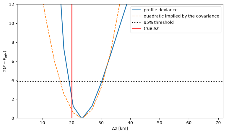
profile   95% [ 18.71,  30.21]
symmetric 95% [ 15.95,  30.70]

The dashed parabola is what the covariance believes. It matches the true curve near the minimum and departs from it further out, falling below on the right and above on the left — so it overstates how far \(\Delta z\) can plausibly fall and understates how far it can rise.

3. Resampling the spectrum

A different question: if the spectrum had scattered differently, what would the fit have returned? sensitivity redraws each spectral value within its uncertainty and refits, many times. It also redraws the centre of any prior, so a prior contributes its own uncertainty rather than acting as a hard constraint.

ensemble = np.array(grid.sensitivity(
    window_size, xpt, ypt, 300, taper=np.hanning, seed=1))

print("            mean      std")
for i, name in enumerate(['beta', 'zt', 'dz', 'C']):
    print("{:>6s}  {:8.3f} {:8.3f}".format(name, ensemble[i].mean(), ensemble[i].std()))

            mean      std
  beta     3.020    0.040
    zt     0.986    0.026
    dz    23.694    2.883
     C     2.399    0.050

4. Markov chain Monte Carlo

The most complete description, and the most expensive: rather than characterising the shape of \(F\) near its minimum, walk over it and collect where the walk spends its time.

metropolis_hastings starts the chain at the mode, proposes moves along the fit covariance from section 1, and tunes the step length during burn-in towards an acceptance rate of 0.234. Proposing one parameter at a time instead would leave the chain unable to move along the ridge, and it would sit still.

posterior, info = grid.metropolis_hastings(
    window_size, xpt, ypt, 20000, 4000,
    taper=np.hanning, seed=1, return_diagnostics=True)
posterior = np.array(posterior)

print("acceptance rate      {:.3f}".format(info["acceptance"]))
print("burn-in acceptance   {:.3f}".format(info["burnin_acceptance"]))
print("distinct states      {} of {}".format(len(np.unique(posterior[0])), posterior.shape[1]))

acceptance rate      0.242
burn-in acceptance   0.232
distinct states      4841 of 20000

fig, axes = plt.subplots(4, 2, figsize=(13, 10),
                         gridspec_kw={'width_ratios': [3, 1]})
truths = [beta_true, zt_true, dz_true, None]

for i, (label, truth) in enumerate(zip(labels, truths)):
    axes[i, 0].plot(posterior[i], lw=0.4)
    axes[i, 0].set_ylabel(label)
    axes[i, 1].hist(posterior[i], bins=50, density=True,
                    orientation='horizontal', color='C0')
    if truth is not None:
        for ax in axes[i]:
            ax.axhline(truth, color='r', lw=1.5)
    axes[i, 1].set_yticklabels([])

axes[3, 0].set_xlabel('iteration')
axes[0, 0].set_title('chain')
axes[0, 1].set_title('marginal')
plt.show()

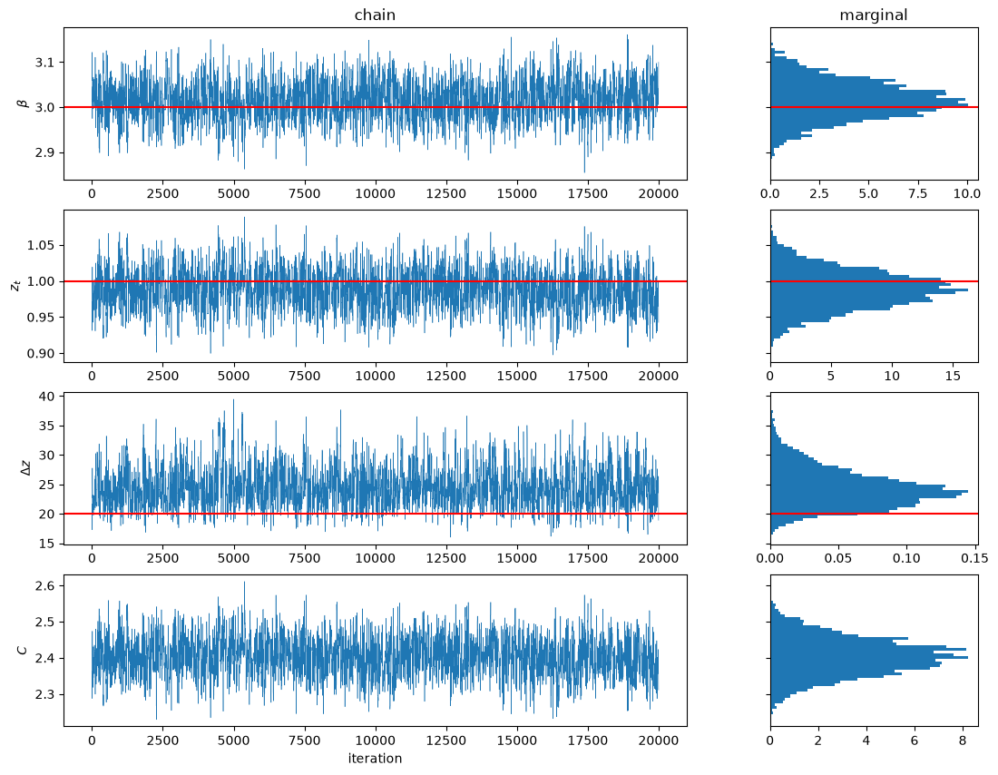
The traces wander across their range rather than drifting or sticking, which is what a chain that is mixing looks like. The marginal for \(\Delta z\) leans right — its mean sits above its median — while \(\beta\) and \(z_t\) are close to symmetric.

Why agreement is not validation

All four methods, on the Curie depth:

CPD, sigma_CPD = grid.calculate_CPD(zt, dz, sigma_zt, sigma_dz)
_, _, cpd_lo, cpd_hi = grid.profile(window_size, xpt, ypt, "CPD",
                                    level=0.95, taper=np.hanning)
cpd_sens = ensemble[1] + ensemble[2]
cpd_mcmc = posterior[1] + posterior[2]

print("                       95% interval        width")
print("covariance +/-2s   [{:6.2f}, {:6.2f}]   {:6.2f}".format(
    CPD - 1.96*sigma_CPD, CPD + 1.96*sigma_CPD, 2*1.96*sigma_CPD))
print("profile            [{:6.2f}, {:6.2f}]   {:6.2f}".format(
    cpd_lo, cpd_hi, cpd_hi - cpd_lo))
lo, hi = np.percentile(cpd_sens, [2.5, 97.5])
print("sensitivity        [{:6.2f}, {:6.2f}]   {:6.2f}".format(lo, hi, hi - lo))
lo, hi = np.percentile(cpd_mcmc, [2.5, 97.5])
print("MCMC               [{:6.2f}, {:6.2f}]   {:6.2f}".format(lo, hi, hi - lo))
print("\ntrue Curie depth    {:6.2f}".format(CPD_true))

                       95% interval        width
covariance +/-2s   [ 16.93,  31.68]    14.75
profile            [ 19.66,  31.22]    11.56
sensitivity        [ 19.93,  31.84]    11.90
MCMC               [ 19.98,  32.88]    12.90

true Curie depth     21.00

fig, ax = plt.subplots(figsize=(9, 5))

ax.hist(cpd_mcmc, bins=60, density=True, alpha=0.5, label='MCMC')
ax.hist(cpd_sens, bins=40, density=True, histtype='step', lw=2, label='sensitivity')
ax.axvspan(cpd_lo, cpd_hi, color='C2', alpha=0.15, label='profile 95%')
ax.axvline(CPD_true, color='r', lw=2, label='true Curie depth')
ax.set_xlabel('Curie depth [km]')
ax.set_ylabel('density')
ax.set_xlim(15, 45)
ax.legend()
plt.show()

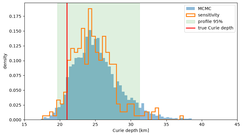
Three of the four agree closely, and every one of them contains the truth. The symmetric interval is the odd one out, and wrongly so: its lower end reaches down to a Curie depth the data rule out.

It would be tempting to read the agreement between the last three as confirmation that they are right. It is not, and this is the most important point in the notebook.

sensitivity redraws each spectral bin independently. metropolis_hastings uses min_func, which sums over bins as though they were independent. They share an assumption, so they agree with each other whether or not that assumption holds — and it does not. A taper spreads each wavenumber over a main lobe several bins wide, so neighbouring bins of the spectrum are correlated; measured over 400 realisations, the correlation between adjacent bins is 0.36 under np.hanning and 0.003 with no taper at all.

The covariance in section 1 corrects for this, which is why its \(\sigma_\beta\) of 0.056 sits about 40% above the 0.040 that the ensembles report. That is not the covariance being conservative. It is the ensembles being narrow.

The only way to tell which is right is to step outside the assumption entirely: generate many independent realisations of the field, fit each, and compare the spread of the results against what each method claimed. Doing that over 200 realisations gives a ratio of true spread to reported \(\sigma\) of 0.997 for \(\beta\), 0.989 for \(z_t\) and 0.991 for \(C\) — the corrected covariance is right, and the ensembles are 30% too narrow. tests/test_bouligand.py keeps that check.

Summary

• The fit covariance is free and is honest for \(\beta\), \(z_t\) and \(C\).

• Use profile for \(\Delta z\) and the Curie depth. Their uncertainty is genuinely asymmetric and a \(\pm\sigma\) misdescribes both ends.

• sensitivity and metropolis_hastings describe the posterior more fully, and MCMC is the only one that gives its shape, but both treat the spectral bins as independent and so report intervals about 30% too narrow.

• Two methods agreeing tells you they share an assumption. Only an ensemble over independent realisations tests whether the assumption is true.

References

Mather, B., & Fullea, J. (2019). Constraining the geotherm beneath the British Isles from Bayesian inversion of Curie depth: integrated modelling of magnetic, geothermal, and seismic data. Solid Earth, 10, 839-850. doi:10.5194/se-10-839-2019

Sambridge, M. (2013). A parallel tempering algorithm for probabilistic sampling and multimodal optimization. Geophysical Journal International, 196(1), 357-374. doi:10.1093/gji/ggt342