Example 4 - Spatial variation of Curie depth

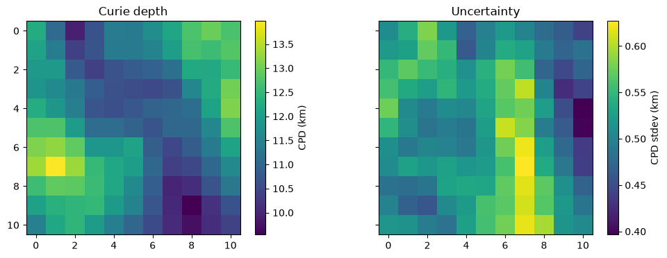
In Examples 2 and 3 we computed the Curie depth at a single point. Here we map it across the magnetic anomaly, with an uncertainty at every centroid.

Contents

• Optimisation routine

• Uncertainty analysis

import numpy as np
import matplotlib.pyplot as plt
%matplotlib inline

import pycurious

# load x,y,anomaly
mag_data = np.loadtxt("../../data/test_mag_data.txt")

nx, ny = 305, 305

x = mag_data[:,0]
y = mag_data[:,1]
d = mag_data[:,2].reshape(ny,nx)

xmin, xmax = x.min(), x.max()
ymin, ymax = y.min(), y.max()

# initialise CurieOptimise object
grid = pycurious.CurieOptimiseTanaka(d, xmin, xmax, ymin, ymax)

Optimisation routine

optimise_routine evaluates optimise at every centroid, distributing them across processors. It takes the same arguments, with lists of coordinates in place of a single pair, and returns one array per output.

The fitting bands are required, in rad/km — there is no default, because a band that is valid for one dataset is rarely valid for another. See Ex2 for how to check a choice with check_bands.

# get centroids

window_size = 200e3
xc_list, yc_list = grid.create_centroid_list(window_size, spacingX=10e3, spacingY=10e3)

print("number of centroids = {}".format(len(xc_list)))

number of centroids = 121

zt_range = (1.257, 1.885)
z0_range = (0.0, 0.628)

zt, z0, zt_int, z0_int, zt_stdev, z0_stdev = grid.optimise_routine(
    window_size, xc_list, yc_list, zt_range, z0_range, taper=np.hanning)

CPD, sigma_CPD = grid.calculate_CPD(zt, z0, zt_stdev, z0_stdev)

print("CPD ranges from {:.1f} to {:.1f} km".format(CPD.min(), CPD.max()))

CPD ranges from 9.5 to 14.0 km

# get dimensions of domain
xcoords = np.unique(xc_list)
ycoords = np.unique(yc_list)
nc, nr = xcoords.size, ycoords.size


# plot results
fig, (ax1, ax2) = plt.subplots(1, 2, sharex=True, sharey=True, figsize=(12,4.))

im1 = ax1.imshow(CPD.reshape(nr,nc))
im2 = ax2.imshow(sigma_CPD.reshape(nr,nc))

fig.colorbar(im1, ax=ax1, label="CPD (km)")
fig.colorbar(im2, ax=ax2, label="CPD stdev (km)")

ax1.set_title('Curie depth')
ax2.set_title('Uncertainty')

Text(0.5, 1.0, 'Uncertainty')

Uncertainty analysis

The map above shows the uncertainty from the fit covariance, which reflects only the scatter of the spectrum. It does not account for the choice of fitting band, which usually matters more.

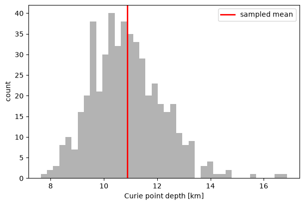
sensitivity resamples the spectrum and jitters both band edges, giving a more realistic spread. It is expensive, so here we run it at a single centroid rather than across the whole grid.

xpt = 0.5*(xmin + xmax)
ypt = 0.5*(ymin + ymax)

zt_s, z0_s, CPD_s = grid.sensitivity(
    window_size, xpt, ypt, 500, zt_range, z0_range,
    taper=np.hanning, band_scale=0.1, seed=1)

i = np.argmin((xc_list - xpt)**2 + (yc_list - ypt)**2)
print("fit covariance only        : {:.2f} +/- {:.2f} km".format(CPD[i], sigma_CPD[i]))
print("including band-edge jitter : {:.2f} +/- {:.2f} km".format(CPD_s.mean(), CPD_s.std()))

fit covariance only        : 10.96 +/- 0.52 km
including band-edge jitter : 10.87 +/- 1.33 km

fig, ax = plt.subplots(figsize=(7,4.5))
ax.hist(CPD_s, bins=40, color='0.7', edgecolor='none')
ax.axvline(CPD_s.mean(), color='r', linewidth=2, label='sampled mean')
ax.set_xlabel('Curie point depth [km]')
ax.set_ylabel('count')
ax.legend()
plt.show()