Example 2 - Compute Curie depth
Tanaka et al. (1999) assume the crust is randomly magnetised between a top \(Z_t\) and a bottom \(Z_b\), which gives a radially averaged power spectrum
where \(k\) is the spatial wavenumber (\(k=2\pi/\lambda\), for wavelength \(\lambda\)) and \(Z_b-Z_t\) is the thickness of the magnetic source.
Rather than fit equation (1) directly, the method takes two limits of it, each of which is a straight line over a different range of wavenumbers.
Short wavelengths. For wavelengths shorter than twice the source thickness the layer looks like a half space, and the second factor tends to 1:
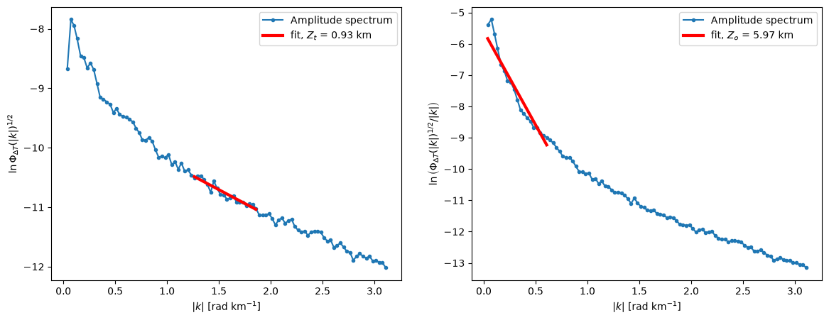
so a straight line fitted here has gradient \(-Z_t\).
Long wavelengths. Equation (1) can be rewritten about the centroid depth \(Z_o\) of the source,
Writing \(d\) for the half thickness, \(Z_t-Z_o=-d\) and \(Z_b-Z_o=+d\), so the bracket becomes a hyperbolic sine:
That last step is an approximation, valid only when \(|k|d \ll 1\). It matters more than it looks, and we return to it below. Dividing through by \(|k|\) leaves a second straight line,
whose gradient is \(-Z_o\). The base of the magnetic source, taken to be the Curie point depth, then follows from the two gradients:
PyCurious fits both lines with scipy.optimize.curve_fit, weighted by the measured scatter of the spectrum, so each gradient carries an uncertainty that propagates through equation (6).
Contents
import numpy as np
import matplotlib.pyplot as plt
%matplotlib inline

import pycurious
# load x,y,anomaly
mag_data = np.loadtxt("../../data/test_mag_data.txt")

nx, ny = 305, 305

x = mag_data[:,0]
y = mag_data[:,1]
d = mag_data[:,2].reshape(ny,nx)

xmin, xmax = x.min(), x.max()
ymin, ymax = y.min(), y.max()
Radial amplitude spectrum
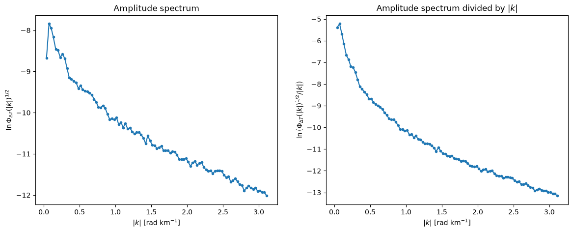
The spectrum is computed from a square window of the magnetic anomaly, using methods that belong to the CurieGrid object.
By default radial_spectrum raises the FFT of the anomaly to the power 2, giving the log power spectrum \(\ln \Phi_{\Delta T}\) that Bouligand et al. (2009) fit. Tanaka’s equations are written in terms of the amplitude spectrum \(\Phi_{\Delta T}^{1/2}\), so here we want power=1.
Wavenumbers come back in rad/km, and the fitting bands below are given in the same units.
The anomaly used here is a synthetic with a known answer: the source sits between 0.305 km and 10.305 km depth, so \(Z_t = 0.305\), \(Z_o = 5.305\) and \(Z_b = 10.305\) km.
grid = pycurious.CurieOptimiseTanaka(d, xmin, xmax, ymin, ymax)

xpt = 0.5*(xmin + xmax)
ypt = 0.5*(ymin + ymax)

window_size = 200e3
subgrid = grid.subgrid(window_size, xpt, ypt)

k, Phi, sigma_Phi = grid.radial_spectrum(subgrid, taper=np.hanning, power=1)

print("{} bins, spaced {:.4f} rad/km, reaching {:.2f} rad/km".format(
    len(k), k[1]-k[0], k.max()))
99 bins, spaced 0.0349 rad/km, reaching 3.11 rad/km
Phi_n = Phi - np.log(k)

fig, (ax1, ax2) = plt.subplots(1, 2, figsize=(14,5))

ax1.plot(k, Phi, '-o', markersize=3)
ax1.set_title('Amplitude spectrum')
ax1.set_xlabel(r'$|k|$ [rad km$^{-1}$]')
ax1.set_ylabel(r'$\ln \Phi_{\Delta T}(|k|)^{1/2}$')

ax2.plot(k, Phi_n, '-o', markersize=3)
ax2.set_title(r'Amplitude spectrum divided by $|k|$')
ax2.set_xlabel(r'$|k|$ [rad km$^{-1}$]')
ax2.set_ylabel(r'$\ln \left(\Phi_{\Delta T}(|k|)^{1/2}/|k|\right)$')

plt.show()
Choosing the two bands
Each straight line is valid only over part of the spectrum:
the \(Z_t\) band needs wavelengths shorter than twice the source thickness, so the half-space approximation behind equation (2) holds;
the \(Z_o\) band needs \(|k|d \ll 1\), the approximation made in equation (4).
Neither condition is visible on the plots above. A band that violates one still yields a confident-looking straight-line fit — just through the wrong part of the curve. check_bands tests a choice explicitly, given a rough guess at the source thickness.
The bands below are the ones this notebook has historically used, converted from cycles/km to rad/km.
zt_range = (1.257, 1.885)
z0_range = (0.0, 0.628)

diagnostics = grid.check_bands(k, zt_range, z0_range, thickness=10.0)
spectral resolution dk = 0.0291 rad/km
zt band: 20 points, wavelengths 3.4-5.0 km
z0 band: 19 points, wavelengths 10.4-166.5 km
z0 band reaches |k|d = 3.04, biasing the Curie depth by about -5.2 km
WARNING: z0_range reaches |k|d = 3.04, which biases the Curie depth low by about 5.2 km. The centroid fit assumes |k|d << 1. Lower the upper edge of z0_range, or use a wider window so there are enough points below it.
Computing the Curie depth
check_bands warns that the \(Z_o\) band reaches \(|k|d \approx 3\), which is not \(\ll 1\), and estimates that this alone drags the Curie depth about 5 km low. Hold that thought until we have a number in hand.
optimise fits both bands and returns the two depths, their intercepts and the standard deviation of each depth, with depths positive downwards. calculate_CPD applies equation (6) and combines the uncertainties in quadrature.
zt, z0, zt_int, z0_int, sigma_zt, sigma_z0 = grid.optimise(
    window_size, xpt, ypt, zt_range, z0_range, taper=np.hanning)

CPD, sigma_CPD = grid.calculate_CPD(zt, z0, sigma_zt, sigma_z0)

print("Top of magnetic source      = {:5.2f} +/- {:.2f} km   (true  0.305)".format(zt, sigma_zt))
print("Centroid of magnetic source = {:5.2f} +/- {:.2f} km   (true  5.305)".format(z0, sigma_z0))
print("Curie point depth           = {:5.2f} +/- {:.2f} km   (true 10.305)".format(CPD, sigma_CPD))
Top of magnetic source      =  0.93 +/- 0.09 km   (true  0.305)
Centroid of magnetic source =  5.97 +/- 0.26 km   (true  5.305)
Curie point depth           = 11.01 +/- 0.53 km   (true 10.305)
mask_zt = np.logical_and(k >= zt_range[0], k <= zt_range[1])
mask_z0 = np.logical_and(k >= z0_range[0], k <= z0_range[1])

fig, (ax1, ax2) = plt.subplots(1, 2, figsize=(14,5))

ax1.plot(k, Phi, '-o', markersize=3, label='Amplitude spectrum')
ax1.plot(k[mask_zt], -zt*k[mask_zt] + zt_int, 'r-', linewidth=3,
         label=r'fit, $Z_t$ = {:.2f} km'.format(zt))
ax1.set_xlabel(r'$|k|$ [rad km$^{-1}$]')
ax1.set_ylabel(r'$\ln \Phi_{\Delta T}(|k|)^{1/2}$')
ax1.legend()

ax2.plot(k, Phi_n, '-o', markersize=3, label='Amplitude spectrum')
ax2.plot(k[mask_z0], -z0*k[mask_z0] + z0_int, 'r-', linewidth=3,
         label=r'fit, $Z_o$ = {:.2f} km'.format(z0))
ax2.set_xlabel(r'$|k|$ [rad km$^{-1}$]')
ax2.set_ylabel(r'$\ln \left(\Phi_{\Delta T}(|k|)^{1/2}/|k|\right)$')
ax2.legend()

plt.show()
Fractal magnetisation
The Curie depth comes out close to the true 10.305 km with a small error bar. That looks like a success, so it is worth checking whether it is one.
Tanaka’s derivation assumes the magnetisation is spatially random. Real crust — and this synthetic — is better described as fractal, which adds a term \(-\tfrac{1}{2}(\beta-1)\ln|k|\) to the log amplitude spectrum. Its gradient is \(-(\beta-1)/2|k|\), so it biases \(Z_t\) high by \((\beta-1)/2\bar{k}\) while leaving the line looking perfectly straight.
This synthetic was built with \(\beta = 3\). Passing beta removes that contribution before fitting.
zt_c, z0_c, _, _, sigma_zt_c, sigma_z0_c = grid.optimise(
    window_size, xpt, ypt, zt_range, z0_range, taper=np.hanning, beta=3.0)

CPD_c, sigma_CPD_c = grid.calculate_CPD(zt_c, z0_c, sigma_zt_c, sigma_z0_c)

print("                      uncorrected   beta-corrected     true")
print("Top      Z_t  [km]   {:8.2f}    {:12.2f}   {:8.3f}".format(zt, zt_c, 0.305))
print("Centroid Z_o  [km]   {:8.2f}    {:12.2f}   {:8.3f}".format(z0, z0_c, 5.305))
print("Curie    Z_b  [km]   {:8.2f}    {:12.2f}   {:8.3f}".format(CPD, CPD_c, 10.305))
                      uncorrected   beta-corrected     true
Top      Z_t  [km]       0.93            0.28      0.305
Centroid Z_o  [km]       5.97            2.73      5.305
Curie    Z_b  [km]      11.01            5.18     10.305
How far can we trust this?
Correcting for \(\beta\) recovers \(Z_t\) almost exactly — 0.29 km against a true 0.305 km, where the uncorrected fit gave 0.93 km. So the correction is doing precisely what the algebra says it should.
But the Curie depth gets worse, falling from 11.0 km to about 5 km. That is the important result in this notebook, and it is not a bug.
Two separate errors were present all along, pulling in opposite directions:
the \(Z_o\) band violates \(|k|d \ll 1\) by a factor of three, which biases \(Z_o\) low;
the unmodelled fractal magnetisation biases both depths high.
In the uncorrected fit these two largely cancelled, which is why the answer looked good. Removing one of them exposes the other. The original agreement with the true value was a coincidence, not a validation — and a coincidence that depended on this particular \(\beta\) and this particular source thickness, so it would not survive on real data.
The honest fix is to narrow the \(Z_o\) band until \(|k|d \ll 1\) actually holds. On this grid that is not possible:
try:
    grid.optimise(window_size, xpt, ypt, zt_range, (0.0, 0.1), taper=np.hanning, beta=3.0)
except ValueError as e:
    print("ValueError:", e)
ValueError: only 2 usable points in the band 0.0-0.1 rad/km, need at least 3. Widen the band, or use a larger window to resolve the spectrum more finely.
A 200 km window resolves the spectrum in steps of about 0.03 rad/km, so a band satisfying \(|k|d \lesssim 0.5\) contains barely two points — not enough to fit a line through. This dataset can constrain \(Z_t\), but it cannot constrain the centroid depth, and therefore cannot constrain the Curie depth either. Resolving a centroid at 5 km depth needs a window of many hundreds of kilometres, so that there are enough long-wavelength bins below the \(|k|d \ll 1\) limit.
tests/test_recovery.py in the source repository demonstrates the method recovering a Curie depth correctly on synthetics generated wide enough to support the fit.
Reporting an uncertainty
The \(\pm\) values above come from the fit covariance alone, and describe only the scatter of the spectrum. They say nothing about where the band edges were placed, which on this data matters far more. sensitivity resamples the spectrum and jitters both band edges:
zt_s, z0_s, CPD_s = grid.sensitivity(
    window_size, xpt, ypt, 500, zt_range, z0_range,
    taper=np.hanning, band_scale=0.1, seed=1)

print("fit covariance only        : {:.2f} +/- {:.2f} km".format(CPD, sigma_CPD))
print("including band-edge jitter : {:.2f} +/- {:.2f} km".format(CPD_s.mean(), CPD_s.std()))
fit covariance only        : 11.01 +/- 0.53 km
including band-edge jitter : 10.87 +/- 1.33 km
fig, ax = plt.subplots(figsize=(7,4.5))
ax.hist(CPD_s, bins=40, color='0.7', edgecolor='none')
ax.axvline(10.305, color='k', linestyle='--', linewidth=2, label='true Curie depth')
ax.axvline(CPD_s.mean(), color='r', linewidth=2, label='sampled mean')
ax.set_xlabel('Curie point depth [km]')
ax.set_ylabel('count')
ax.legend()
plt.show()
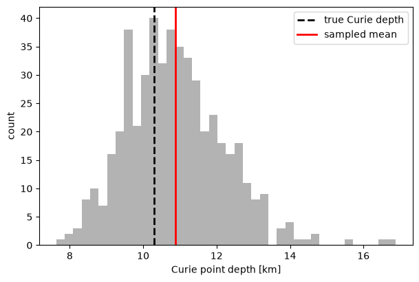
Widening the error bar in this way is more honest, but it still does not cover the two systematic biases discussed above: those shift both fits coherently rather than scattering them, so no amount of resampling will reveal them. Only check_bands, and a source model appropriate to the data, can.
Summary
Fit the \(Z_t\) band where wavelengths are shorter than twice the source thickness, and the \(Z_o\) band where \(|k|d \ll 1\). Use
check_bandsrather than assuming.Pass
betaif the magnetisation is fractal, which for real crust it generally is.Treat the fit covariance as a lower bound on the uncertainty, and
sensitivityas a better one.An answer that matches expectation is not evidence that the bands were valid.